Boundary Value Problem (BVP) Solver
This project addresses a 2D boundary value problem defined on a square domain with two removed circular areas. The solution is obtained using finite element methods (FEM), which involves triangulating the domain and computing the stiffness matrix. The BVP is defined as follows:
\[ \nabla \cdot \left( e^{-\beta(x,y)} M(x,y) \nabla u \right) = 0, \quad (x,y) \in \Omega \]
\[ \frac{\partial u}{\partial n} = 0, \quad u \in \Gamma_N \]
\[ u(\partial A) = 0, \quad u(\partial B) = 1 \]
Integral Equation Formulation
To get the integral equation formulation for this Boundary Value Problem, I applied the Green's Identity and followed similar steps in the lecture notes. I have also used the knowledge from S. Larsson (2009), Partial Differential Equations with Numerical Methods.
\[ \int_{\Omega} \nabla u e^{-\beta(x,y)} M(x,y) \nabla u \cdot dx = 0 \]
Let \( u = v + u_D \) where \( v \) is the free nodes, and \( u_D \) are nodes on the boundary.
\[ \int_{\Omega} e^{-\beta(x,y)} M(x,y) \nabla u \cdot \nabla v \cdot dx + \int_{\Omega} e^{-\beta(x,y)} M(x,y) \nabla v \cdot u_D \cdot dx = 0 \]
Domain Description
The domain Ω is the square \([-1, 1]^2\) with two removed circles A and B of radii 0.2 centered at \((-0.5, -0.1\sin(0.5\pi))\) and \((0.5, 0.1\sin(0.5\pi))\), respectively.
Triangulation Result
Using the module for discritization of trianglation mesh, I have created the triangulation plot for the domain \([-1, 1]^2\) in below (Figure 1).
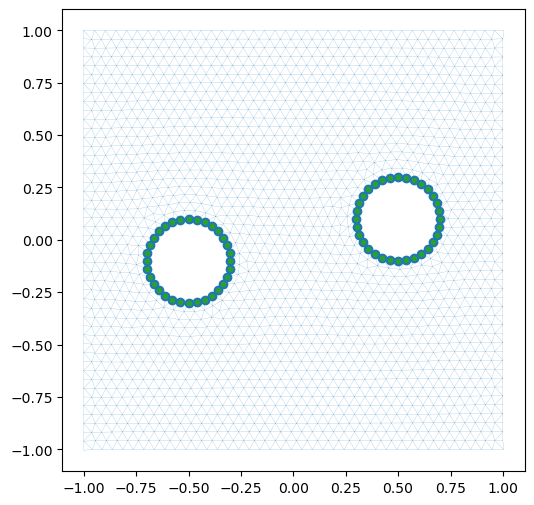
Figure 1: Triangulation plot for the domain \([-1, 1]^2\). In total, there are 1909 number of points, and 3582 number of triangles.
Methodology
To solve this equation, it is required to handle two extra terms: one is the scalar function \( V(x, y) \), and the other is the matrix function \( M(x, y) \). The scalar term is easier to deal with, where we need to multiply the result of the stiffness by a scalar, which is similar to what was done in assignment 8. If we ignore the matrix term, we will get a result like the following (Figure 2). Dealing with the matrix term is in a different approach; I handled the matrix term in the stiffness matrix.
\[ \text{stima} = \frac{|T|}{2} \cdot G \cdot M(x, y) \cdot G^T \]
After applying the term, the result pattern kind of shifts depending on the positions of \( x \) and \( y \) (Figure 3).
Final Result
Below is the final result of the BVP solution:
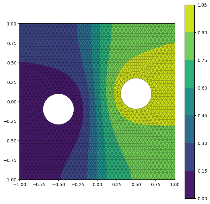
Figure 2: The solution of finite elements when ignoring the matrix term.
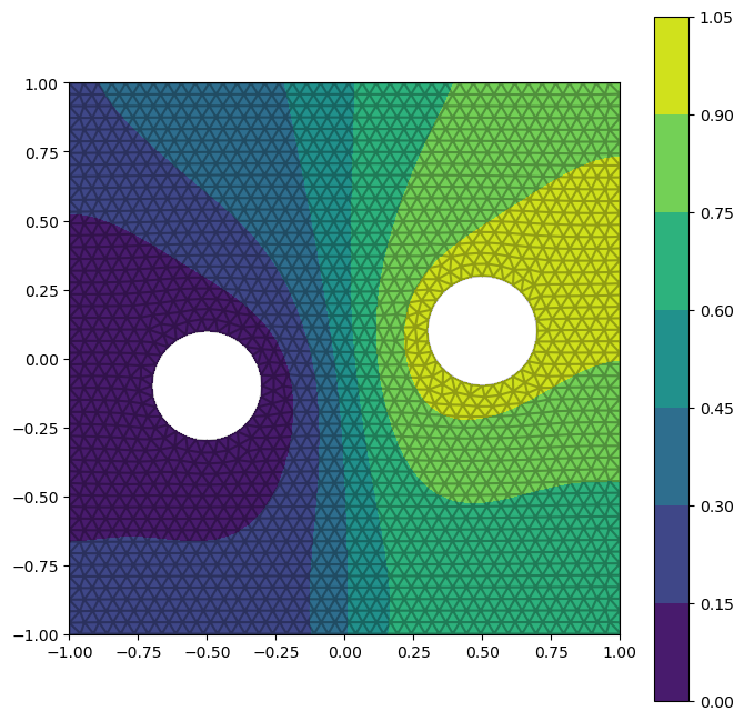
Figure 3: The solution of finite elements after introducing the matrix term.