Optimal Interpolation for Point Vortex System
This project implements Optimal Interpolation (OI) to assimilate drifter observations into a nonlinear point vortex model with 2 vortices and 1 drifter. The goal is to understand how well a simple OI scheme can correct forecast errors and track the chaotic truth trajectory. The framework developed here allows us to validate analysis against truth and no-DA baselines, while assessing the sensitivity to background-error covariance Pb.
Point Vortex Model
Each vortex is a point singularity with circulation \(\Gamma\) embedded in incompressible, inviscid 2-D flow. Vortex coordinates \((x_j,y_j)\) evolve via:
while a passive drifter \((\xi_k,\eta_k)\) obeys analogous equations forced by the vortices:
where \(\ell_{jj'}^2=(x_j-x_{j'})^2+(y_j-y_{j'})^2\) is the squared separation distance between vortices and \(\ell_{kj}^2=(\xi_k-x_j)^2+(\eta_k-y_j)^2\) is the squared separation between drifter and vortex.
This system exhibits several interesting properties that make it challenging for data assimilation. The point vortex model conserves total circulation, energy, and angular momentum in the absence of external forces, creating a constrained dynamical system. Even with just two vortices, the motion of drifters can be chaotic, showing sensitive dependence on initial conditions—small differences in starting positions can lead to dramatically different trajectories over time. Additionally, the system demonstrates non-normal growth characteristics where small perturbations can lead to rapid error amplification due to the nonlinear interactions between vortices and drifters.
Experimental Setup
| Parameter | Value |
|---|---|
| Vortex circulation \(\Gamma\) | 1 |
| Initial vortex positions | (1,0), (-1,0) |
| Drifter initial position | (1.0,-0.6) |
| Forecast span | \(T=(4\pi)^2\) |
| Time step | \(\Delta t = 1\) |
| Initial error | \(e^a_0 \sim \mathcal{N}(0, 0.01^2)\) |
| Observation noise | \(\epsilon^t_k \sim \mathcal{N}(0, 0.02^2)\) |
Optimal Interpolation (OI)
The analysis update is given by:
Only drifter positions are observed, so the observation operator is:
I initialize Pb and R as diagonal matrices with \(\sigma_b=\sigma_o=0.02\):
Validation Example
To validate the OI implementation, we can examine a specific analysis step. For instance, at \(k=5\):
Background State \((\mathbf{x}^b_5)^\top\):
[0.799, -1.001, 0.062, 0.141, 0.882, -0.565]
Observation \(\mathbf{y}_5^\top\):
[1.210, -0.370]
Innovation \((\mathbf{d}^{OI}_5)^\top = (\mathbf{y}^o_5 - H\mathbf{x}^b_k)^\top\):
[0.328, 0.195]
Kalman Gain \(\mathbf{K}^{OI}\):
Since \(H \mathbf{P}^b H^\top = \mathbf{R}\), then \((H \mathbf{P}^b H^\top + \mathbf{R})^{-1} = \frac{1}{2} (H \mathbf{P}^b H^\top)^{-1}\)
\(\mathbf{K}^{OI} = \begin{bmatrix} 0 & 0 \\ 0 & 0 \\ 0 & 0 \\ 0 & 0 \\ 0.5 & 0 \\ 0 & 0.5 \end{bmatrix}\)
Analysis State \(\mathbf{x}^a_5\):
[0.799, -1.001, 0.062, 0.141, 1.046, -0.467]
Notice that only the drifter components (last two elements) are updated, while vortex positions remain unchanged. This highlights the limitation of our diagonal \(\mathbf{P}^b\) formulation.
Results
OI dramatically reduces forecast error and keeps the drifter trajectory close to truth:
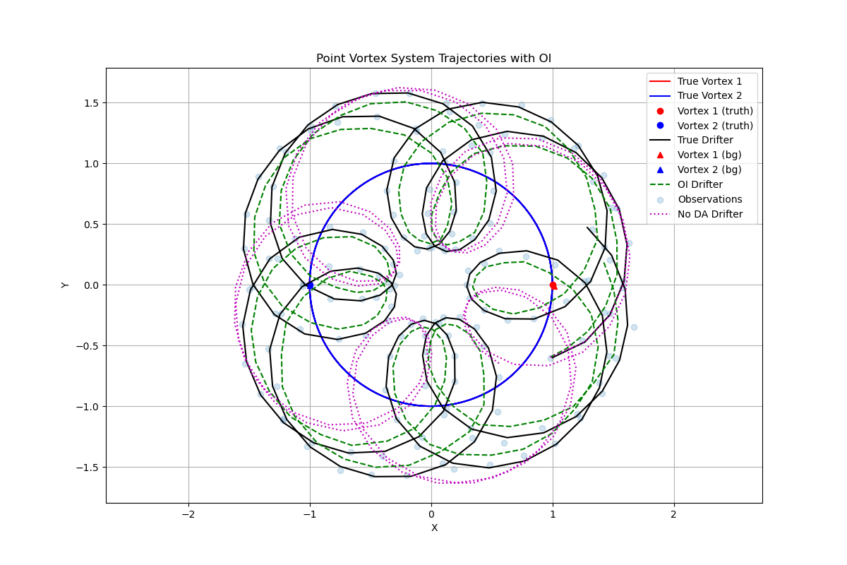
Figure 1: Truth (black), NoDA (magenta), and OI analysis (green) trajectories. The OI analysis successfully tracks the true trajectory despite the chaotic nature of the system, while the no-data-assimilation forecast quickly diverges.
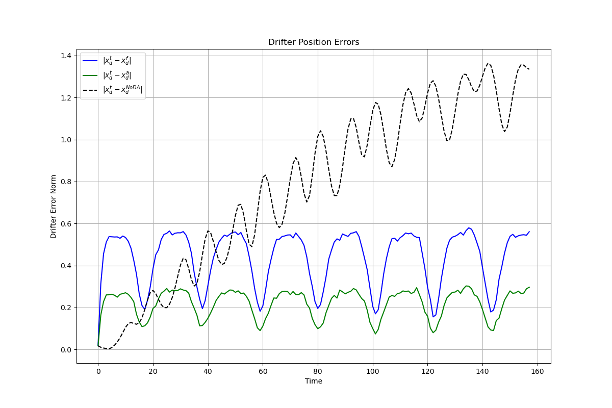
Figure 2: Drifter error norms—analysis (green) consistently outperforms forecast (blue) and no-DA (dashed). The analysis errors remain bounded throughout the assimilation window, demonstrating the effectiveness of OI in constraining the system state.
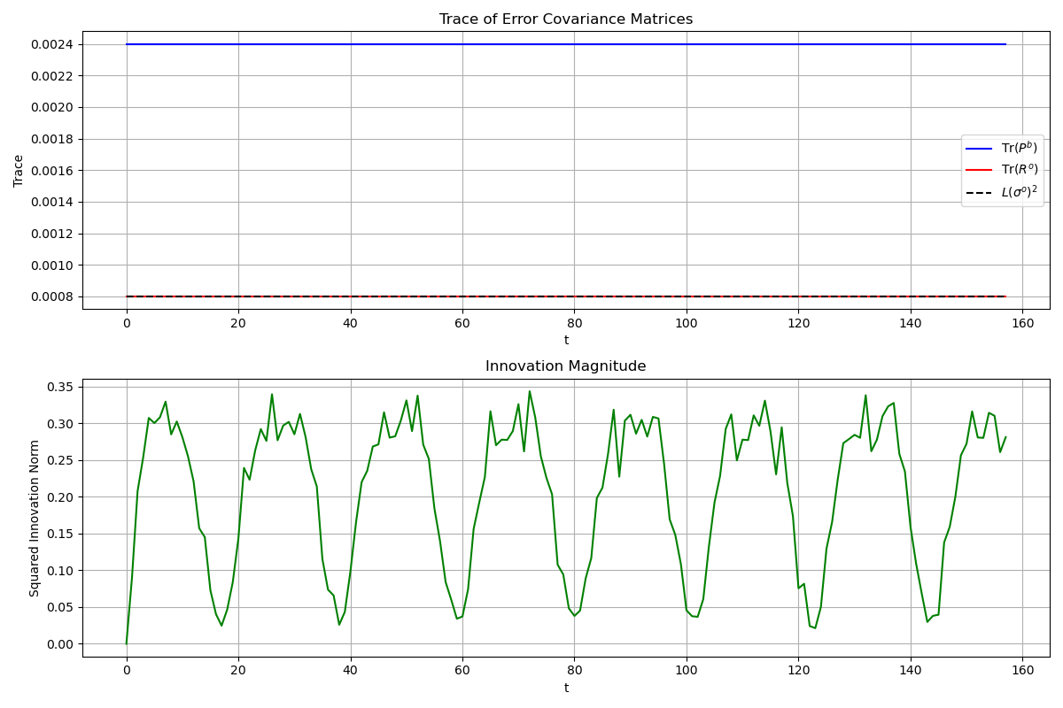
Figure 3: Top panel shows the trace of background error covariance (\(\mathbf{P}^b\)) and observation error covariance (\(\mathbf{R}\)) matrices compared to the theoretical limit \(L(\sigma^o)^2\), where \(L=2\) is the observation space dimension. Bottom panel displays the squared innovation norm \(||d^{ob}_k||^2\) measuring the magnitude of the difference between observations and background forecasts.
Tuning Pb
Smaller background variance tightens the Kalman gain, but under-estimating Pb can degrade performance. I compare two alternative configurations: \(\mathbf{P}^b = (0.01)^2\mathbf{I}\) (small) and \(\mathbf{P}^b = (0.04)^2\mathbf{I}\) (large).
Figure 4a: System trajectory with small background error covariance \(\mathbf{P}^b = (0.01)^2\mathbf{I}\). The smaller background errors result in weaker corrections, causing the analysis to follow the forecast more closely.
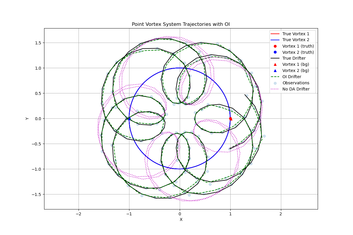
Figure 4b: System trajectory with large background error covariance \(\mathbf{P}^b = (0.04)^2\mathbf{I}\). The larger background errors lead to stronger corrections, allowing the analysis to track observations more closely.
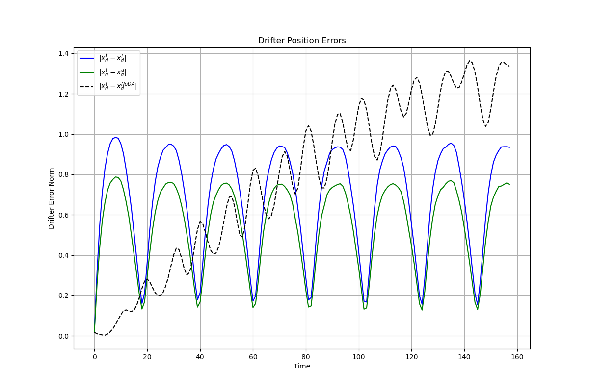
Figure 5a: Drifter errors with small background error covariance. The analysis errors (green) show less improvement over the forecast errors (blue), indicating suboptimal assimilation.
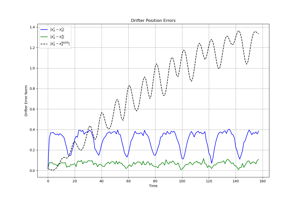
Figure 5b: Drifter errors with large background error covariance. The analysis errors are significantly reduced compared to the forecast, showing more effective assimilation but potentially overfitting to noisy observations.
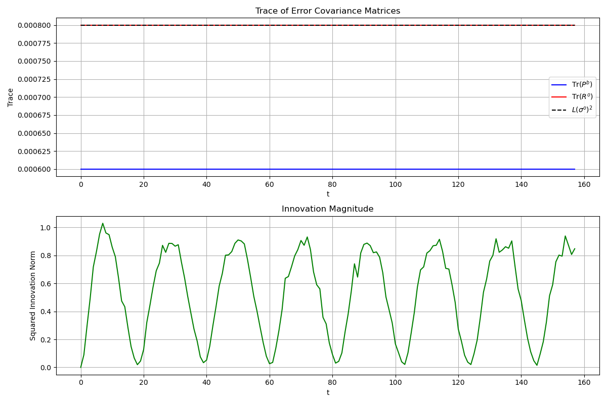
Figure 6a: Innovation statistics with small background error covariance. The innovations are consistently larger than expected, indicating potential filter divergence due to underestimated background errors.
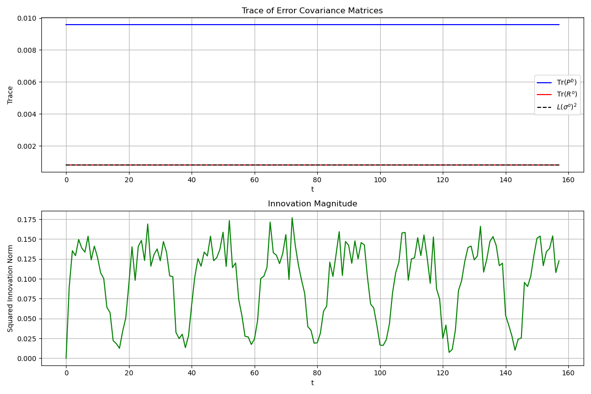
Figure 6b: Innovation statistics with large background error covariance. The innovations are smaller than expected, suggesting potential over-confidence in the observations relative to the background.
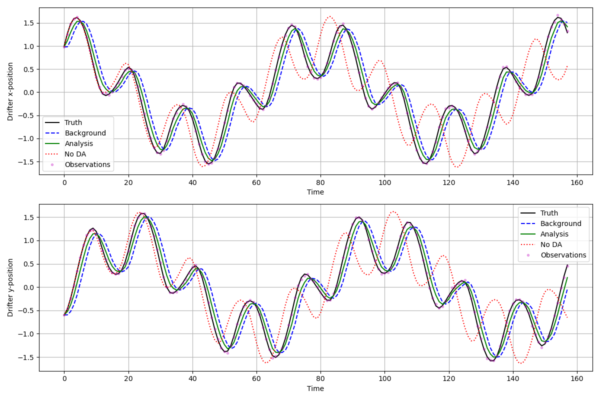
Figure 7: Verification of drifter position timeseries with truth data. This time series shows the x and y components of the drifter positions over time, comparing truth (black), analysis (green), and forecast (blue) trajectories. The analysis successfully tracks the oscillatory behavior of the true drifter path.
Discussion
OI performance depends critically on proper specification of Pb and R. Testing revealed that our configuration (Pb = R = (0.02)2I) shows good innovation consistency, while underestimated Pb significantly reduces Kalman gain effectiveness. The chaotic nature of vortex dynamics leads to rapid breakdown of linearity, making the practical assimilation window significantly shorter than expected, though drifter-only errors remain manageable even with longer windows. Tangent Linear Model (TLM) validation tests conducted during this study revealed that linearity assumptions became invalid much faster than anticipated due to the strongly nonlinear vortex interactions.
Static diagonal Pb misses critical vortex-drifter cross-correlations, which fundamentally limits the long-term predictability of the system. In physical reality, vortex positions directly govern drifter motion, so the true background error covariance should contain off-diagonal elements representing these relationships. Instead of the diagonal structure used in this study, a more physically realistic covariance would include cross-correlations:
The current implementation means the Kalman gain cannot translate drifter observations into vortex position updates, resulting in suboptimal analysis where only drifter positions get corrected while errors in unobserved vortex positions continue to grow. This is particularly limiting because vortices dominate the system dynamics, and small vortex position errors can lead to large drifter forecast errors over time.
The fixed Pb used in this study cannot capture error growth from nonlinear dynamics. The relationship between vortex and drifter positions is inherently nonlinear, with partial derivatives describing these interactions:
These derivatives represent the fundamental relationships that should be reflected in the background error covariance, but are entirely missed by our diagonal formulation. In the present framework, with H = [02x4 I2x2], the resulting Kalman gain has a specific structure:
This structure means innovations can only correct drifter positions, never updating the more dynamically important vortex components. With a flow-dependent covariance that included cross-correlations, the Kalman gain would likely have non-zero elements in the upper rows, allowing drifter observations to correct vortex positions.
Potential improvements could come from using Extended Kalman filter (EKF) or ensemble methods (EnKF) to estimate cross-correlations between vortex and drifter positions, or implementing adaptive covariance inflation to maintain filter stability. A hybrid approach combining a static climatological component with flow-dependent correlations might also help address the fundamental limitations identified here. Despite these limitations, the linear OI scheme still provides significant short-term error reduction, demonstrating the value of even simple data assimilation in highly nonlinear systems. This project underscores the fundamental challenge in data assimilation: balancing model and observational uncertainties while accurately representing their interdependencies.
References
- Aref, H. (2007) Point vortex dynamics: a classical mathematics playground. J. Math. Phys., 48:065401.
- Ide, K., Kuznetsov, L., Jones, C.K.R.T. (2002) Lagrangian data assimilation for point vortex systems. J. Turbulence, 3.
- Kuznetsov, L., Ide, K., Jones, C.K.R.T. (2003) A method for assimilation of Lagrangian data. Mon. Wea. Rev., 131(10):2247-2260.